Recently, I've been working on inventsummer, a part of inventXYZ. It's run by my friend and some of his classmates, and I highly suggest checking them out - they're doing great things. Either way, given this was written when the Coronavirus outbreak was happening, it's unsurprising that one of the projects in inventsummer revolved around it. Specifically, we were guided through building a stochastic simulator for modeling the spread of a virus in a city. The model itself was very simple, but it still showed some important features of virus transmission.

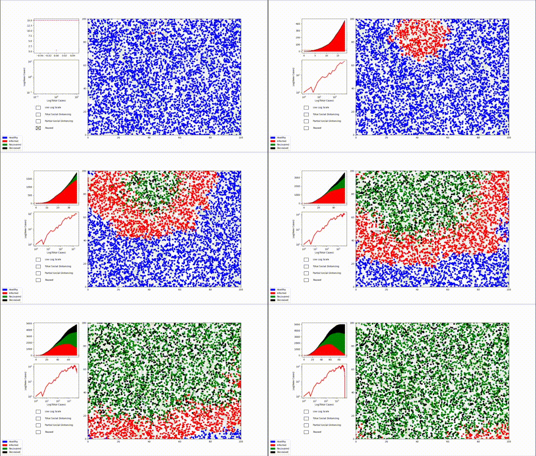In particular, the curve of the total number of affected people to date resembled a logistic curve. However, it's highly unlikely the curve was actually logistic. For instance, it seemed new cases only formed at the boundary of the "blob" of current cases. This is especially aparent toward the end of the spread, where the boundary was just the "frontier" between the top and bottom sides of the arena. One can imagine this playing out in an arena that is much taller than it is wide. There, cases would grow linearly, not logistically, for most of the spread.

As you may have guessed, I've recently been interested in modelling the spread of viruses, at least with many simplifying assumptions in place. Specifically, I'd like to fit differential equations to the spread, mainly because I know they can and have been used to model stochastic processes like Browinian Motion. I've done some work on a model similar to inventsummer's, and I may blog my work when it's more complete. For now, though, I'd like to write about a much simpler case.

I assumed that we had a total population size of @@K@@ and denoted the current number of infected people as @@k \leq K@@. I further said that every infected person had some probability @@P_I@@ of infecting a given healthy person in the next second. Note that, once a person was infected, they remained so for the duration of the spread - there was no recovery. Also see that I completely ignored individual differences in @@P_I@@ - I said that it's the same for every pair of infected and healthy people, regardless of how much prior contact they've had.

Those assumptions, though extremely limiting, allow us to solve explicitly. Using the common probability "trick" for the union of independent events and assuming that our numbers are large enough for probabilities to be treated as proportions, we see that the average rate of increase in the infected population will be %% \frac{\text{d}k}{\text{d}t} = \left(1-(1-P_I)^k\right)\cdot(K-k) . %% This can intuitively be arrived at by assuming @@k@@ doesn't change much over the next second and computing what the effect would be. Of course, @@k@@ does change over the couse of that second, so our computation would only be the rate of change at that instant - the derivative with respect to time.

The above differential equation doesn't seem to be solvable with elementary methods. But, just as we can approximate @@\sin x \approx x@@ for small values of @@x@@, we can also apply a first order approximation to the function %%\begin{align*} (1-P_I)^k &= \exp(\ln(1-P_I)\,k) \nl &\approx 1 + \ln(1-P_I)\,k \nl 1 - (1-P_I)^k &\approx -\ln(1-P_I)\cdot k . \end{align*}%% Thus, for sufficiently small @@P_I@@, we get %% \frac{\text{d}k}{\text{d}t} = -\ln(1-P_I)\cdot k\cdot(K-k), %% the classic logistic differential equation.

Note that the logic in the above few paragraphs is slightly more nuanced than what I present. Indeed, this creates some issues for me later on. See if you can spot the issue before I get to it.

Of course, this all works in theory, but what about in practice? To test, I wrote a very simple Python script to simulate forward stochastically and compare with the predicted results. The code is basically what you'd expect, so I won't include a listing here, and I'll just link to it at the end of this post. The only slightly complicated part involves computing the probability @@P_i@@ of a given infected person infecting a fixed healthy person in one timestep instead of in one second. To do this, we again apply the probability "trick" for the union of independent events to get %%\begin{align*} P_I &= 1 - (1-P_i)^\frac{1}{\text{d}t} \nl P_i &= 1 - (1-P_I)^{\text{d}t}, \end{align*}%% assuming we're using natural units so @@\text{d}t@@ is in seconds.

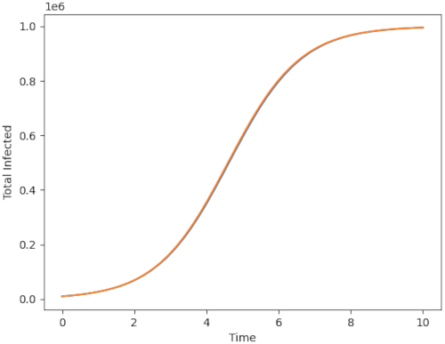Overall, the plot came out quite nicely. The simulation was run for @@10\,\text{seconds}@@ with:

• @@\texttt{POP_SIZE} = K = 10^6@@,
• @@\texttt{P_INFECT} = P_I = 10^{-6}@@,
• @@\texttt{DT} = \text{d}t = 10^{-2}\,\text{seconds}@@, and
• @@\texttt{PROP_INITIAL_INFECTED} = 1\%@@ of the initial population infected.

The orange curve is the expected number of infected people at a given time, and the blue curve is the actual number. Note that the former is an overshoot of the latter in the above image. At first, I thought this was random variation, but it was actually fairly consistent behavior. However, decreasing @@\text{d}t@@ fixed this issue.

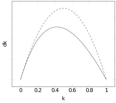
Having confirmed my model in a nominal case, I wanted to see what happened when I violated the assumption that @@P_I@@ was small. Plotting the change in the number of infected people versus the total number infected, we'd expect a slow but present divergence from the "ideal" parabola. I decided for no particular reason to set @@P_I = 75\%@@, which would give the plot below, where the dotted line is the "ideal" parabola and the solid line is the "actual" curve.

Of course, just cranking up @@P_I@@ didn't exactly yield the best results. Combining that, with the fact I kept the population size high to minimize random artifacts, meant that everyone got infected almost immediately. Remember that, in my model, everyone is "on top of each other." To compensate for this, I reduced the total simulation time to @@10^{-5}\,\text{seconds}@@. I also reduced @@\text{d}t@@ to not lose resolution, but I didn't want to set it so low that we introduce too many random artifacts into the plot of the derivative. After some trial and error, I set @@\text{d}t = 2.5\cdot 10^{-9}\, \text{seconds}@@.

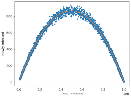The above image was the result of my experiment. The orange curve is the "ideal" parabola, and the blue points are the actual data I collected. I was surprised to see no loss in accuracy due to my "small-probability approximation," and it turns out that's because of the nuance in my reasoning I mentioned earlier. It seems that it's best to assume that @@k@@ only remains (relatively) constant over the course of a single timestep. Over that step, %%\begin{align*} \text{d}k &= \left(1 - (1-P_i)^k\right)\cdot(K-k) \nl &= \left(1 - \left(1-\left(1-(1-P_I)^{\text{d}t}\right)\right)^k\right)\cdot(K-k) \nl &= \left(1 - (1-P_I)^{k\,\text{d}t}\right)\cdot(K-k), \end{align*}%% where we just substituted in what we got earlier for @@P_i@@ and did some algebra. Now, we can assume that @@k\,\text{d}t \leq K\,\text{d}t@@ is small (as it will be in the limiting case), and expand to the first order as %%\begin{align*} \text{d}k &= -\ln(1-P_I)\,k\,\text{d}t\cdot(K-k) \nl \frac{\text{d}k}{\text{d}t} &= -\ln(1-P_I)\cdot k\cdot(K-k). \end{align*}%% It's the same result, just different reasoning and weaker requirements.

That basically wraps up my exploration with this simplified model. There are many situations where it starts to break. I already pointed out one at the start of this post, but another one would be where @@\text{d}t@@ is large. Consider a scenario where people go to the supermarket once a week but otherwise isolate. In that case, the actual growth would be much less than what this model would predict just given the probability of transmission.

Nonetheless, it makes sense that we see logistic-like growth in all kinds of virus spread. Not only does the basic logic - that new cases come from old cases and that the growth will cap at some point - hold, but we might also be able to compute then use an average @@P_I@@ for the population. Indeed, in real life, we do compute a population-wide average for %% R_0 \approx \frac{1}{1-P_I}, %% even though individual @@R_0@@s can vary wildly. It seems this simple logistic model is more versatile than I give it credit for.

Resources

• Code for this post
• Simulator for inventsummer